Technical Manual for Rapid Inundation Mapping

Executive Summary

The Rapid Inundation Model (RIM) tool is an on-demand inundation map building tool developed by the MMC to support the United States Army Corps of Engineers (USACE) water control management mission. This mission encompasses the regulation of river flow through more than 700 reservoirs, locks, and other water control structures located throughout the nation. The inundation layers housed in the RIM tool database are derived from models developed under the Corps Water Management System (CWMS) National Implementation Plan. CWMS is an integrated system of hardware and software that allows hydrometeorological, watershed, and project status data to be viewed through a user-friendly interface which allows water managers to evaluate and model the watershed. The RIM tool is intended to compliment the CWMS suite of software by allowing decision makers to create sophisticated maps quickly and disseminate them to others within USACE and to emergency managers.

The RIM tool is an on-demand inundation map building tool developed by the MMC to support the United States Army Corps of Engineers (USACE) water control management mission. This mission encompasses the regulation of river flow through more than 700 reservoirs, locks, and other water control structures located throughout the nation. The inundation layers housed in the RIM tool database are derived from models developed under the Corps Water Management System (CWMS) National Implementation Plan. CWMS is an integrated system of hardware and software that allows hydrometeorological, watershed, and project status data to be viewed through a user-friendly interface which allows water managers to evaluate and model the watershed. The RIM tool is intended to compliment the CWMS suite of software by allowing decision makers to create sophisticated maps quickly and disseminate them to others within USACE and to emergency managers.

The intent of the RIM tool is to provide a rapid inundation map within minutes of obtaining forecasted stages for key areas within the watershed. The tool is designed so that inundation near a key critical gage will reflect the forecasted stage and then, using that same flow to project the stage at that location, an approximate inundation will be reflected throughout the river reach upstream and downstream using selections based on the team's knowledge and understanding of where a break point between gages should occur. The further away from the gage, the less accurate the inundation layer may become, but it may still provide value in flood inundation estimates where timing is critical. The tool is not meant to supersede a more accurate CWMS inundation map or United States Geological Survey (USGS)/National Weather Service (NWS) maps that are calibrated to higher standards but is meant to provide the first estimate of inundation during an event. In some cases, where the basin response may be very flashy, the tool may benefit the CWMS modelers who cannot produce inundation mapping within the response time required. It may also benefit CWMS watersheds that require extensive River Analysis System (HEC-RAS) computation times to produce inundation mapping by providing inundation layers that are already computed. Engineering judgment should always be used to provide the best available quality-controlled layers within the given time constraints for each watershed prior to distribution.

Section 1 - Data Collection

Data collection is an important step in the beginning phase of any project. The modeler should work with the district staff to obtain all necessary data and model files, as described in this section. It is important that this work be completed prior to the kickoff meeting, so that a productive kickoff meeting will occur, and all participants understand the scope of the work and the required effort it will take to complete the project.

Section 1.1 - Quarterly Introductory Webinar

At the beginning of each quarter, the PM will schedule an introductory webinar where the H&H technical lead will demonstrate the RIM tool for project teams slated to start during that respective quarter. Example projects will be shown and modeling lessons learned will be discussed from other projects. A link to the RIM tool is available at https://prod.mmc.usace.army.mil/mmc/ The H&H technical lead will show how to select a project then proceed to show how the reaches and slider bars work. The demonstration will discuss why the tool was created, how it can be used, the goals and purpose of the tool, and what the future benefits of using the tool will allow, as well as limitations. General concepts of the creation and how the scripting works for the tool will also be discussed. The H&H technical lead will introduce the concept of reach polygons and discuss best practices set forth in Appendix C . The GIS lead will review the project spreadsheet and instructions set forth in Appendix B. The consequences lead will present an overview of the methods for deriving the consequences data as described in Section 5. Finally, the PM will review the standard operating procedures laid out in this document, particularly focusing on the data collection requirements and the designated milestones.

Section 1.2 - Project Folders

Figure 1-1 is an example of the MMC folder structure. The Geographic Information System (GIS) team member creates the MMC folder structure in the MMC file share: \\wpc-netapp3.eis.ds.usace.army.mil\RMCSTORAGE5\Production\RIM. Team members experiencing access issues can contact the MMC Mapping and Documentation Branch Chief or the MMC Documentation Production Lead to request access.

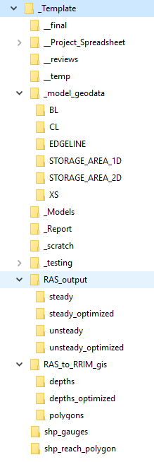
Figure 1-1. MMC-RIM Project Folder Template

Section 1.2.1 - Template Folder and Subfolder Contents

The template folder stores the folder structure used when creating a new project and contains the subfolders identified in Sections 1.2.2–1.2.5.

Section 1.2.2 - _model_geodata Folder and Subfolder Contents

The model geodata folder stores GIS-formatted geometries from the RAS model not including the flood extent.

Section 1.2.3 - _testing Folder and Subfolder Contents

The testing folder stores the high and low flows used by the consequences and GIS team members to prepare for the data processing once the complete dataset is provided. This folder structure mimics the RAS_output and the RAS_to_RIM_gis folders and subfolders.

Section 1.2.4 - RAS_output Folder and Subfolder Contents

The RAS_output folder stores the RAS Model depth grids. The subfolders “steady” and “unsteady” are for the type of output for that particular basin. The “optimized” folders stores any post-processing of the data such as down sampling, compression, and merging raw output.

Section 1.2.5 - RAS_to_RRIM_gis Folder and Subfolder Contents

The RAS_to_RRIM_gis folder stores the GIS processing output used for the final loading. Subfolders “depths” and “polygons” store the processed raster depth grids and polygons that are sliced per each reach_polygon reach. The “optimized” folder stores any post-processing of the data such as down sampling, compression, and merging output.

Section 1.3 - Project Spreadsheet

The project spreadsheet houses all watershed, modeling, geographic information system (GIS) data, and consequences data for the life of the project. The GIS lead sets up a project spreadsheet template when setting up the project folders. Data collected prior to the kickoff meeting is captured in the project spreadsheet following the instructions provided on the readme tab and Appendices A and B. This spreadsheet is located in the _Project_Spreadsheet folder in the team’s project folder.

Section 1.4 - Projections

The standard projection for all MMC projects is as follows:

• USA_Contiguous_Albers_Equal_Area_Conic_USGS_version.
• Linear units are set to U.S. feet.
• The MMC Production Center will use North American Vertical Datum of 1988 (NAVD 88) for all elevation data.
• The MMC projection is used throughout the RIM layers development process.
• Detailed projection parameters are provided in Section 4.1.1.

Section 1.5 - Terrain

All terrain files are identified by the districts located within the watershed. The terrain files used should reflect the best available data used for CWMS implementation. If the district obtains more accurate terrain, the team will discuss in the kickoff meeting how to appropriately incorporate those adjustments into the RIM tool layer development. Models will not be funded to update geometries from existing CWMS geometries, but some benefits of using more accurate terrain may better reflect inundation boundaries and could be incorporated into the terrain used for layer development. Caution and engineering judgment should be used to ensure inundation layers will most accurately reflect and not contradict CWMS inundation map products.

Section 1.6 - Existing Models and Reports

The modeler works with the district’s water management staff to obtain the most current model(s) of the study watershed. This should include HEC-RAS and Reservoir System Simulation (HEC-ResSim) models developed under the MMC CWMS National Implementation Program. It is crucial that the modeler work with district staff, as the most up-to-date models may vary from those initially developed under the CWMS program. The modeler should also obtain and review all reports that explain the development and calibration of those models. The modeler should also identify any watershed studies that include profile development such as Federal Emergency Management Agency (FEMA) flood insurance studies (FIS) or other frequency profile studies. The team should also identify any inundation mapping products created for the watershed that can be used to calibrate the inundation map boundaries from historic events of known flows and inundation extents from MMC maximum high (MH) pool breach inundation boundaries from reservoirs within the watershed.

Section 1.6.1 - Model Version

The district informs the modeler which version of HEC-RAS is being used to run the model. The model should run in HEC-RAS 5.0 or higher, though exceptions may be made in special circumstances approved by the H&H technical lead. The modeler may need to run the model in a more recent version of HEC-RAS and will have to correct any issues with the model to fix any error messages that may arise. Coordination with the district may be needed during this process.

Section 1.6.2 - Model Calibration and Stress-Testing

The modeler should review the current state of the HEC-RAS model. Calibration runs should be checked and results verified, and if any issues are found they should be noted and addressed during the kickoff meeting. The model should also be stress-tested to ensure it can handle extreme high flows such as a PMF breach flow for any reservoir within the system.

Section 1.6.3 - Model Runtimes

The modeler should run several events to determine how long it will take on average to run one event through the model. A low flow, medium flow, and high flow should all be run to calculate the average runtime for the model. Prior to the kickoff, the PM will request the model runtimes from the modeler, as it will be used to develop the schedule and budget for the project.

NOTE

When running HEC-RAS two-dimensional (2D) models, additional model runtime sensitivity should be performed using different numbers of computing cores to determine the optimal number of cores required to reduce runtimes. This can be done by running a one-hour computation simulation in multiple copies of a plan then adjusting the computational cores used for each plan, running the simulation, and checking the timing of the simulation. Utilizing the lowest number of computational cores that provide the same runtimes may allow the team to run multiple plans on one computer and speed up the creation of modeled inundation layers.

Section 1.7 - Gage Data

The other important information that the modeler needs to gather prior to the kickoff meeting is gage data. Gage locations help the team determine how the model and model results will be broken into reaches for the RIM tool. It is important that the modeler take the time to work with the district water management staff to identify all relevant gages within the study watershed at this time. All gages within the watershed should be identified so the team can determine which ones will be used for the project. Gages may be used from USACE, USGS, NWS, or other gage sources identified by the district. Ideally, the gages need to have a webpage, such as NWS AHPS, where the RIM tool can access the (forecast) data to enhance visual selection of data during use of the tool. In special circumstances, not all gages may have this data and can be manually adjusted if needed. All gage data needs to be filled out in the project spreadsheet template provided in the _Project_Spreadsheet folder. See Appendix B for guidance on populating this spreadsheet. The district provides the modeler with a shapefile showing the locations of all relevant gages within the study watershed. This should include any locations where the end user would need to adjust flood stages (as slider bars) to produce the rapid inundation maps through the online tool. The district should cross check the gage shapefile with the locations of the common computation points (CCPs) within the HEC-ResSim model to ensure no gages were overlooked.

Section 1.8 - Draft Reach Polygons

The watershed is broken down into smaller reaches to allow users to customize inundation and flow combinations throughout the watershed. The entire team should have input as to how these reaches are determined. Hydrologic Modeling System (HEC-HMS) subbasins and HEC-ResSim gages and junction points can be used as a starting point, but the final reaches do not need to correspond to those polygons. In the final product, users are able to specify a flow or stage for a given reach and see the corresponding inundation and consequences that would result from that flow. See Appendix C for more information. The modeler works with the H&H technical lead to develop a first draft of a reach polygon shapefile using guidance from Appendix C. A template shapefile is in the shp_reach_polygon folder with the necessary fields included.

Section 1.9 - Project spreadsheet model info, gage metadata, and Curves

The modeler gathers the model info such as version information and model types, gage information, and the most current rating curves for all relevant gages identified in Section 1.7, with the assistance of district water management staff. Rating curves for reaches will have USACE data and for gaged reaches will also include USGS or other agency data. This data is important later in the project, as it is used to tie model results to gage readings for final display within the online mapping tool. This information needs to be added to the template project spreadsheet. If the model is unsteady, the interpolation spreadsheet should be utilized and should reference the raw curve data and extract the exact flows for the profiles produced. See Appendix B for guidance on populating this spreadsheet.

Section 1.10 - Base Schedule and Budget

A base schedule and budget are developed by the PM based on the run time determined in Section 1.6.3. The project schedule and budget are sent to the district point of contact (POC) and the H&H modeler for feedback before the kickoff meeting.

Section 2 - Project Kickoff Meeting

Section 2.1 - Project Kickoff Meeting

The MMC PM schedules a project kickoff meeting after the draft schedule and budget is developed. At a minimum, the invitees will include: the district POC(s) (water management staff), the H&H technical lead, the H&H team lead, the GIS lead, the consequences lead, the PM, and the assigned modeler.

The kickoff meeting is held to clarify the scope of the study as well as the schedule and budget. The RIM H&H team lead and modeler will discuss key technical information with the district personnel. Primary data sources gathered during data collection, such as existing hydraulic models, high-resolution terrain, reservoir locations, gage locations, existing profiles, existing inundation maps, and project datum conversions, will also be reviewed.

Section 2.2 - Review Data Collected

Data collected in Section 1 is documented in the project spreadsheet and reviewed via webinar during the kickoff meeting. It is the responsibility of the GIS lead to ensure team members understand how all project data and reviews should be recorded in the project spreadsheet over the life of the project.

Section 2.2.1 - Available Models

All available models will be discussed in the kickoff meeting. These could include, but are not limited to, CWMS HEC-RAS models, MMC dam breach HEC-RAS models, district HEC-RAS models, etc. Once all models are identified, the team will discuss the pros and cons of using each model. The team will decide which of the available models would best meet the intent in creating inundation mapping products to support the tool that was displayed during the tool demonstration. In general, models should be calibrated to an acceptable quality, but, if model calibration is not available, the best available model should be used. The final set of models used for the study should be identified in the final report for the project to allow future users to understand which models were used for the study and why.

Section 2.2.2 - Critical Gages

Once model extents are determined in the kickoff meeting, based on best available models selected for use with the project, the modeler reviews the area for all pertinent stage and/or flow gages. The modeler should discuss with the district’s water management office to help determine which gages are most relevant for the area of interest during the kickoff meeting. Gages relevancy may be determined on multiple factors. Examples of questions that may be used to determine these factors include: is it a forecast gage, is it currently maintained, does it have stage/flow data or a rating curve at that site, is it a tributary gage or a main stem gage, do we have a consequence area nearby that requests mapping frequently?

If the water control staff is not available to help with this information during data collection, it can be obtained from best available sources, most gage data is available online. Gage data can be obtained from using online sources for purposes of discussion during the kickoff meeting but must be verified by the water control staff as they are the key end user of the tool once it has been fully developed. It is mandatory that the water control staff attend the kickoff meeting and concurs with the development of the project before proceeding with model development and final polygon reach boundary location selections. Typically, gage locations and their corresponding data can be found through the USGS, NWS, or Rivergages websites.

This is a critical step in the RIM tool creation because the user uses these gages in the creation of the map. For example, the user looks at forecasted stages on NWS plots and uses those stages for each reach polygon within the RIM tool to select the appropriate inundation map layer.

Section 2.2.3 - Review Reach Polygons

Prior to the kickoff meeting, the modeler delineates draft reach polygons as described in Section 1.8. During the kickoff meeting, the team reviews and revises the reach polygons based on the watershed characteristics and the guidance provided in Appendix C. Minor changes to the reach polygons are made during the webinar. Final reach polygon review occurs after modeling begins as described in Section 3.3.

Section 2.3 - Modeling Strategies

Just as flow ranges vary from study to study, so may the form of hydraulic computation for each study. This is determined at the modeler’s discretion or discussed with the team if the modeler is uncertain. The RIM tool is designed to be a first cut or rough inundation map while a more accurate inundation map is being formed. It is possible that the model may have more than 100 scenarios depending upon the flow range and increment selected. With this in mind, if the model does not contain 2D elements, it is preferable for the project to use steady flow simulations. Using steady flow is the most conservative answer. When the RIM tool provides emergency managers a first cut map, it is better for it to be on the conservative side. If the model contains 2D elements, it will be necessary to use unsteady flow.

Section 2.3.1 - Flow Ranges

Each modeled basin will have a varying range of flows that are appropriate for that watershed. For instance, if the user is modeling a large river, the lowest flow modeled for the study may be 200,000 cubic feet per second (cfs) with the higher limit being 2,000,000 cfs. On the opposite hand, if one is studying a small stream, the range may be between 500 cfs to 5,000 cfs.

To determine the higher and lower limits of the flow range for each model, a good rule of thumb is to start with channel capacity or action flood stage, whichever is lowest, and extend to a high range of a probable maximum flood (PMF) with breach. If model extents are cut off prior to reaching a PMF breach condition of the largest reservoir influencing the tributary being modeled, capturing flow conditions that extend to the highest possible extent allowable using the final selected model is encouraged. District water management staff should advise the modeler on the minimum stage/flow value of concern is for each river within the watershed. For the higher limit, a PMF breach is stated, but the modeler will have to use engineering judgment to determine the greatest possible flow that could come through the system. If there are multiple reservoirs within the model, the modeler determines which is most likely to produce the highest flows during a PMF breach event. Once these limits are determined, it is best to run those flows through the model and provide the results to the consequence and GIS personnel as described in Section 3.1. These limits are used in the setup of each RIM tool project.

Selection of flow ranges are set by the smallest flow needed on the smallest tributary and the largest flow needed from PMF breach outflow from any reservoir within the watershed. All tributaries have the minimum to maximum flow ranges computed for water surface profile creation, but, when setting each reach’s specific flow range based on the gage, the range can be limited to the most credible values needed for that gage.

Section 2.3.2 - Flow Increments

The modeler must determine the increments at which flows will increase within the model to get from the lower limit to the higher limit. Rating curves at gage locations are typically used to help determine this. Commonly, a district or emergency manager is interested in a stage, not a flow. As a result, the flow increment is based upon what stage increase the district staff deem appropriate for a river. In some areas, such as a flat, wide floodplain, two tenths of a foot may make a vast difference in flood extents or impacts, whereas in steep areas, one foot may be more reasonable. The end goal is that the RIM tool has a map that can be rounded to the nearest future flood event within a basin. At gages, it is important to capture a more refined stage increment from action flood stage to major flood stage. Once that threshold is exceeded, larger flow increments can be utilized for higher, less frequent stages in order to maintain a reasonable number of scenarios.

NOTE

Each HEC-RAS reach within the model may have a different flow increment based on its geometry. The smallest flow increment will dominate the determination of flows selected. As the stage increases, the flows can be adjusted to higher flow values to replicate the flow increment desired.

Once the stage increment is settled, the modeler can go to the rating curves on the corresponding river and determine what flow will cause that amount of increase in stage. The modeler can follow the rating curve from the lower limit to the higher and begin creating plans for that set of flows. Each gage has to be carefully evaluated for the appropriate flow increment for that location. After all flow increments are identified, the modeler selects the smallest flow increments to be applied to the entire watershed. If the rating curve does not extend to the higher limit, the modeler takes the last flow increment recorded and repeats.

Once completed for each stream of interest, the flow increments could combine to more than 100 scenarios. Again, this will be different for each study and a reasonable number of flow increments should be selected to capture the appropriate stage increase desired. For example, if a one-foot stage increment is needed, look at the entire system of rating curves and determine the minimum flow change to achieve that increment. Once that value is obtained, flows can be increased to maintain that one-foot stage increment for the watershed.

Section 2.4 - Unique Issues

All watersheds and areas may have unique issues that arise. The kickoff meeting is a good time to discuss any unique issues with the modelers from the district. Unique issues could include how to handle key confluences, ungaged areas, interpolation, and one-dimensional (1D) versus 2D modeling needs. This information is recorded as assumption, issue, etc. in the template project spreadsheet available in the tool. See Appendix B for guidance on populating this spreadsheet.

Section 2.5 - Team Roles and Responsibilities

Detailed descriptions of the roles and responsibilities of each team member are in the MMC Technical Manual for Program Management. The PM discusses the roles and responsibilities of each team member and the district. District involvement during the entire project is essential for success.

Section 2.6 - Budget and Schedule

The project schedule and budget are discussed to ensure all parties involved in the modeling and review process understand the timeframes for milestone completion and allotted funding for each team member. Revisions, as necessary, are made during the kickoff. The H&H team lead will invite the H&H modeler and district POC to join the biweekly RIM conference calls following the kickoff meeting to ensure the project is progressing on schedule and resolve any outstanding issues. District involvement in the RIM conference call is encouraged. If for some reason a modeler or district cannot attend, the modeler will provide an email update to the PM and H&H team lead highlighting progress, tasks accomplished, and any questions that require follow up from the PM or H&H team lead.

Section 3 - Hydraulics and Hydrology Modeling

The H&H modeling section covers the essential process for utilizing existing HEC-RAS models to generate water surface profiles for various selected flow increments. The H&H modeler uses the best available models as discussed in the kickoff meeting to generate the required layers and perform the analysis listed in this section. The reviews incorporated in this section are critical to the success of the project and are designed to minimize any rework required for multiple computational runs. The goal of generating sample flows is to establish the higher and lower bounds for the system to evaluate and update the polygon extents. This also provides the modeler a chance to become familiar with the model prior to conducting a lot of time-consuming runs. Once the sample flows are established, the team will review the data and verify if the current path forward is acceptable. Any modeling tweaks should be made after the sample flows review to prevent additional rework. The section also describes naming conventions and the process for incorporating various model types such as steady flow, 1D unsteady flow, and 2D flow models. In addition, guidance on unique issues are listed as well, such as how to handle tidal flow situations, model validation, rating curve extraction, and how to transfer data to the GIS and consequence team members. If questions arise that are not covered by this document, users should reach out to their H&H team lead for assistance.

Section 3.1 - HEC-RAS Model Description

All models created for the MMC Production Center will include a thorough description field that provides potential users with pertinent information. The following items will be listed in the HEC-RAS Model Description field:

• Basin
• Project Type
• Location of Basin/Extent
• General Description of Modeling Approach
• Modeling Date
• Program and Version
• Vertical Datum and Units
• Horizontal Datum and Units
• Horizontal Projection
• MMC Hydraulic Modeler
• MMC RIM Team Lead
• District H&H Contact Person
• Date of Last Modification
• "Controlled Unclassified Information"

Section 3.2 - Generate Sample Flows

Initial model runs will utilize the higher and lower flow limits determined in Section 2.3.1. These initial runs will help the modeler determine if the model is stable during a low-flow run and an extreme high-flow run. The high-flow range will be set by looking at the highest peak outflow from all of the existing dam breach studies for projects in the watershed. The largest flow would dictate and control the high flows set for steady flow models. Unsteady and 2D models will consider reasonable high flows for each tributary based on a project-specific basis due to the model split between main stem and tributaries. To reduce extra plan creation, high flows for tributaries without upstream reservoirs should be set to reasonable PMF-type non-breach conditions. If there is a dam on that tributary, the PMF breach flow condition still applies.

To generate sample flows for a steady model, the modeler should use the model selected in the kickoff meeting and create one new steady flow file and plan file for steady flow models. The flow file will include only two profiles for all reaches in the model and all flows will be set to the minimum and maximum established flow for the watershed. Once computed, the extents will be checked to ensure the cross sections are wide enough to capture all inundation. Geometry extensions should be minimal and if it is a significant amount of work, the H&H technical lead should be consulted.

To generate sample flows for an unsteady 1D or 2D model, the modeler should use the model selected in the kickoff meeting and create a minimum of two new unsteady flow files and plan files. The flow files will include one for low flow and one for high flow. Additional plans may be required depending on tributaries within the model as well. If the model has significant tributaries, the best practice is to run a set of two plans for the main stem river reach and then a second set of two plans to account for all tributaries. Once the plans have been computed, the extents will be checked to ensure cross section and/or 2D flow areas are sufficient to capture all inundation. Geometry extensions should be minimal and if it requires significant work to fix, the H&H technical lead should be consulted.

Section 3.3 - Review Inundation and Polygons Extents

Upon completion of the initial model runs, the modeler should review the model output. First, the results from the high- and low-limit model runs should be analyzed within RAS Mapper to see if there are any abnormalities within the depth grid/inundation extents. Analyze these results just as if they were going to be released to the public. Issues to look for include, water extending to the edge of a cross-section/storage area, significant depth change across terrain boundaries, water surface extrapolation for cross-sections/storage areas, if the inundated area is reasonable, if leveed areas are correct, etc. Once the inundation is clear of abnormalities, the modeler checks the elevation relationship versus the terrain or topographical map in the cross-sections nearest to each gage location. The modeler can also check to ensure the rating curve produced for the low flow resembles values that line up with the USGS rating curves. If the model is very far off, the model calibration from existing model should be checked. The model may still be used, but the H&H team lead should be consulted and documentation of the discrepancy should be noted in the final report and should suggest that future model improvement may be beneficial. Because most models should have been calibrated prior to this study, the discrepancies should not be too significant and should not be common.

Once the modeler has deemed the initial inundations accurate, the modeler will export the depth grid for each of the higher and lower limit runs and bring them into Aeronautical Reconnaissance Coverage map (ArcMap). The purpose here is to assess the inundations in relation to the reach polygons and gage locations originally created.

• Does the inundation fully fit within the bounds of the reach polygons?
• Does the original reach polygon layout seem adequate for the inundation?
• Should one reach be extended because it more accurately represents the area than the next polygon?
• Is there a major slope change and the reach should be split to better represent the area? Appendix C details information on delineating reach polygons.

Section 3.4 - Sample Flows Review

Review is an extremely important part of the MMC production process. Several review steps are required to ensure the inundation consistently represents all project scenarios and accurately represents the consequences associated with each scenario. A review checklist housed within the project “_reviews” folder will be used to track comments regarding aspects that are checked through the review process. The project spreadsheet remains with the model and is used throughout the entire review process (i.e., district webinar review, and final review).

Before creating all the additional plan files, the modeler holds a webinar with the H&H technical lead, H&H team lead, consequences technical lead, GIS technical lead, and district POC to review items in the review spreadsheet. The review tab captures items to be reviewed during this meeting, including but not limited to the following:

• What are the results from low-(channel capacity or action flood stage) and high-(PMF breach) flows?
• Do reach polygons capture the full inundation extent?
• Are the flow range and increments still appropriate for this watershed?
• Do the FEMA FIS profiles resemble the same slope?
• Were kickoff selections used according to the PWP?

Following the district webinar review, the modeler will revise the high- and low-flow scenarios if deemed necessary by the review team. The modeler then uploads the project spreadsheet and depth grids produced in the sample flow runs to the RAS_output folder within the project folder structure on RMCStorage5 and sends an email notifying the GIS and consequences team members. The GIS team uses these initial inundations to begin coding the reaches within the RIM tool. The consequences team needs to use these inundation extents/depth grids to begin modeling the consequences within Flood Impact Analysis Model (HEC-FIA). The consequences team specifically needs the low-flow channel capacity/action flood stage inundation extent, so, if the lower limit is not the channel capacity scenario, then it must be modeled as well. Finally, the modeler shares run times with the PM and H&H technical lead via email and they will reevaluate the schedule and budget for the remainder of the project.

Section 3.5 - Steady Modeling

Steady flow modeling should be considered for areas where there is a well-defined terrain, attenuation is not critical, and there are not flat areas where the flood would sprawl for miles. Steady flow will be the quickest and most robust modeling option to produce these rapid flood layers and should be taken into consideration first.

There will be one plan, one geometry, and one flow file set up for steady modeling. Within the flow file the modeler should rename all the profiles with the associated flow (e.g., PF1, PF2, PF3, etc. become 100, 1000, 10000). The “PF#” or profile name is represented by the flow ranges desired. Further discussion in Section 2.3.2 discusses the appropriate flow increment based on all gage locations and rating curves for the watershed. first.

Developing additional flow profile runs that may seem unreasonable for small tributaries or large tributaries is not an issue for the tool development. The modeler should select only the resulting water surface profiles that satisfy the minimum, maximum, and appropriate incremental flow regime profiles for each reach polygon. The remaining flow scenario outputs are discarded or ignored all together when selecting the appropriate slider bar settings in the RIM tool. This allows the tool to use only the user-specified range and values that would be appropriate for the reach polygon. Only action flood stage to PMF breach type flow conditions are represented in the slider bars allowing control of inundation layers shown. Therefore, very small flows on significant tributaries can be hidden within the tool along with very large unrealistic flows for small tributaries.

Section 3.6 - Unsteady and Two-Dimensional Modeling Setup

Modeling unsteady simulations for a RIM watershed will not require any special geometry changes relative to a common CWMS model simulation. The major difference between unsteady RIM study simulations and other unsteady simulations are the model flow inputs. Each study is different, but many study models include a main stem river with a number of tributary rivers. For a RIM study, the modeler separates plan and flow files as main stem, tributary 1, tributary 2, tributary 3, etc.

For main stem model runs, first save the plan name, short ID, and flow file name to the corresponding flow rate for the main stem river. The flow rates modeled are the ones determined in Section 2.3.2. The modeler then inputs a flow hydrograph on the upstream cross-section of the main stem river. The first timestep should begin at a normal flow and slowly ramp up the flows (depending on the model, this may be several days) to hit the desired flow for that run. Then, hold that flow constant for a long enough period for the peak flow to reach the most downstream cross-section. Figure 3-1 depicts an example of this.

While creating the main stem river plan and flow files, tributaries need to be considered. The modeler sets all tributary inflows to a minimal flow rate for that river, essentially adding just enough flow for the model to remain stable without adding substantial flow to downstream reaches. Tributary inflow remains constant for the entirety of all main stem model simulations. This allows a single model run to represent a single flow rate for the entire main stem river. For example, consider the first main stem model run to be 25,000. If 25,000 cfs is input at the upstream cross-section, the downstream cross-section should remain as close as possible to 25,000 cfs. In a typical basin, modelers should aim for 500 cfs or less difference between the inflow hydrograph and the most downstream cross section on the main stem river. If tributaries added substantial flow, the upstream cross-section flow would be 25,000 cfs and the downstream cross-section could end up being 100,000 cfs. For proper RIM tool mapping, it is critical for each run to represent a single flow.

Once main stem simulations are completed, the modeler can run each tributary simulation. All tributaries included in the CWMS model should be considered for incorporation into the RIM tool inundation layers. The modeler approaches these simulations with the same process. Save the plan name, short ID, and flow file name with initials for tributary and corresponding flow rate. Set flows for the tributary to ramp up to the desired flow rate and set all other reaches, including the main stem reach, to minimum flow.

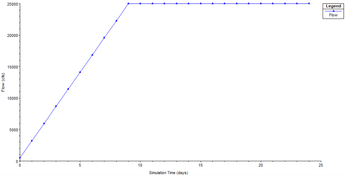
Figure 3-1. Unsteady Flow Hydrograph

Section 3.7 - Validate Model

Model validation is a key step in the process. The modeler should pull in a profile from a previous study and compare to the profiles generated for a nearly similar stage event. Meaning the modeler goes to the key gaged location of interest within the reach polygon. For example, look at a FEMA FIS profile for the 100-year flow and know what stage that produces, then pull up the RAS created stage profile for that same stage (keep in mind, the flows may be off slightly due to geometry changes not matching the FEMA model). One should check the slope of this profile, key consequence areas, whether bridges matter, and do any adjustments need to be made for a few of these different profiles.

The model should be validated to a minimum of three events: high flow, near period of record flow or 100-year, and near channel capacity.

Section 3.8 - Develop Plans and Naming

Naming convention is critical for RIM studies as the GIS team needs to easily read them into the process. Since there may be hundreds of plans, it is essential for them to be clearly named to reduce the time in the scripting process.

The default RAS output should be utilized ensuring a full integer flow without commas is used in the name of the output depths as opposed to using a P1 for a profile. If it is absolutely required to use a profile name instead of flow value, such as when you are modeling a system that includes different reaches with drastically different flow regimes, a legend of the values and how they correspond to the flow for each reach shall be provided through a crosswalk within the project spreadsheet. The crosswalk within the project spreadsheet will provide information for the tool to link the profile name to the proper flow regime on each reach within the HEC-RAS geometry.

File and Folder Names:

• Steady output: Steady flow output should be named “Depth ([flow in CFS]).[NAME OF TERRAIN].tif” as shown in Figure 3-2. The flow value in the output file name shall be integer form at the agreed upon flow increment including specified equal intervals OR at flows determined to equate to a certain water surface elevation and must match the rating curves provided. The name of the terrain will be unique per RAS model. A consistent name for every depth grid is the default for entire output.

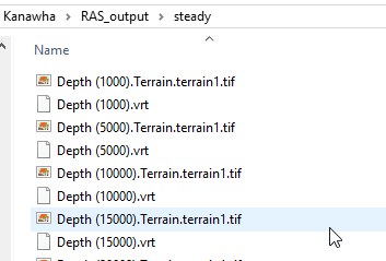
Figure 3-2. Steady Flow Profile File Naming Example

• Unsteady output: Folder names should indicate the flow and, therefore, the grid file name does not need to contain flow but needs to have a generic name that is the same for all folders. Folder names should indicate the full integer value and avoid using kcfs or k as shown in Figure 3-3. Output files for tributaries should contain an identifier code prior to the flow value in the name. If multiple models are utilized, the folder name should contain the prefix for that model location. A crosswalk of which folder prefix corresponds to which reach should be documented in the project spreadsheet. Details are provided in Appendix B.

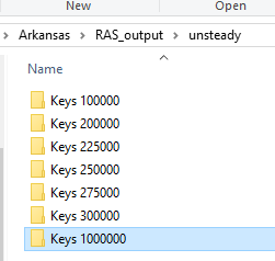
Figure 3-3. Unsteady Flow Profile Inundation Folder Name Example 1

In Section 2.3.2, the modeler chose the specific flows that would be run in the model. If using steady flow, the profile name should match the flow amount. If the run uses 1,000 cfs, the profile name should be “1000.” Figure 3-2 shows an example of this. If using unsteady flow, the plan name, short ID, and flow file should be named with each corresponding flow amount. If the run uses 25,000 cfs, plan name, short ID, and flow file will be named “25000.” Figures 3-3 and 3-4 depict this. Be cognizant to exclude all symbols and spaces.

If the model at hand contains tributaries, the same methodology is used for steady flow. View Figures 3-5 and 3-7. For unsteady flow analyses, the modeler will need to add an identifier to each plan name, short ID, and flow file. For instance, if the modeler is running a simulation using 5,000 cfs for the Bogue Chitto River tributary, the plan name, short ID, and flow file will be named “BC5000.” Figures 3-6 and 3-8 depict this.

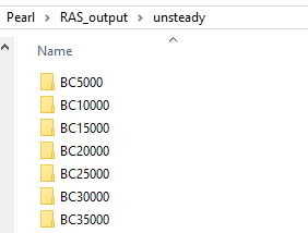
Figure 3-4 Unsteady Flow Profile Inundation Folder Name Example 2

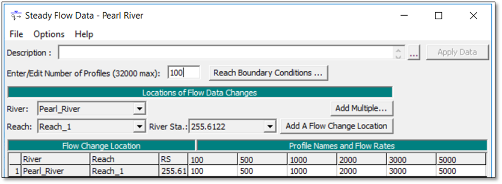
Figure 3-5. Steady Flow Data Naming Convention

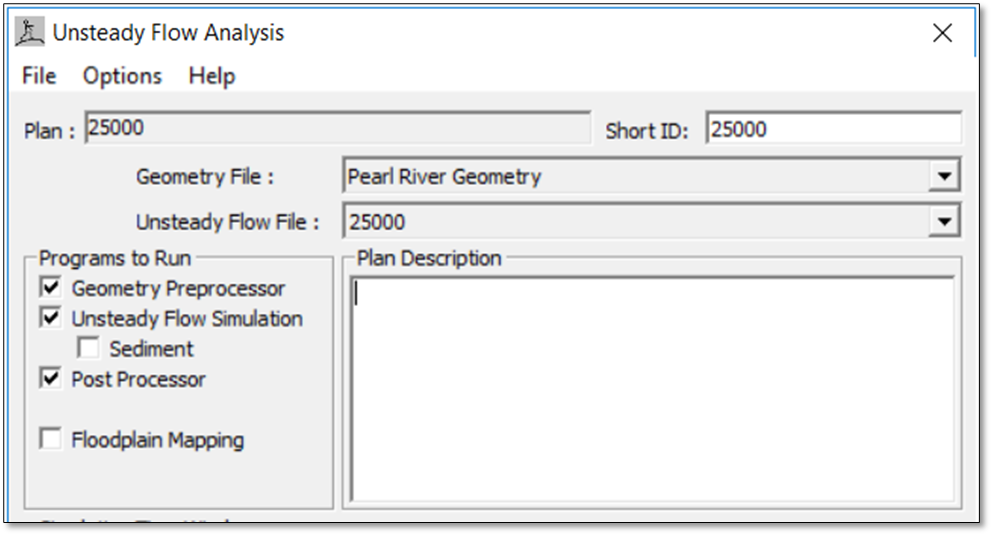
Figure 3-6. Unsteady Flow Plan Naming Convention

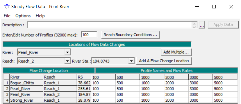
Figure 3-7. Steady Flow Data with Tributaries

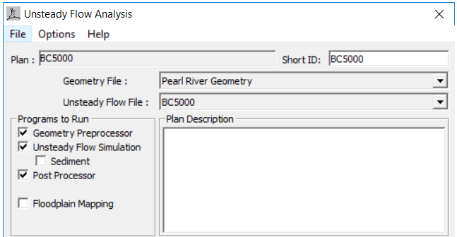
Figure 3-8. Unsteady Flow Plan Naming Convention for Tributaries

If questions arise, the modeler works with the GIS team to ensure proper naming convention for each model profile or plan is used. Modelers should work with the GIS team on the front end so nothing requires renaming on the back end of the modeling effort.As for the deliverables, the modeler only needs to export max depth grids for each profile or plan run.

When a depth grid is saved in RAS Mapper, it saves under the short ID name within the RAS model folder. The modeler copies the entire folder for each plan run to deliver to the GIS and consequences team.

Section 3.9 - Storm Surge Simulations

The RIM tool includes storm surge inundations if a study model includes a coastal basin. The exception to this is if there are no population centers or areas of interest that could be impacted by storm surge. These will be simple simulations that represent any possible storm surge event for that area. The modeler uses the same model or creates a quick 2D HEC-RAS model for the area that would be impacted by storm surge. In most cases, the modeler chooses to use the same geometry as used for all other simulations. To ensure the effects of inundation are based on storm surge, ensure all main stem and tributary inflows are near normal flow, so it does not greatly expand the inundation of the storm surge.

Determine the range of storm surge events by either viewing historical data for downstream gages, or if the gages are not sufficiently downstream, use a National Oceanic and Atmospheric Administration (NOAA) tidal gage station near the project area. If the modeler can find a long period of record for stages, use the highest event and add ten feet to get the upper limit of storm surge simulations. Alternatively, the NOAA tidal gage station publishes the historic maximum water level in the Station Home Page. If using a NOAA gage, note the datum used, as their website typically defaults to reporting the maximum water level in MHHW (highest tide) and it must be converted to NAVD 88.

For example, if during a recent hurricane, a gage recorded a storm surge of 9.9 feet, set the upper limit of storm surge simulations to be 20 feet. The lower limit will be when flooding first begins to occur, likely the Mean Higher High Water (MHHW) scenario. These limits will be at the discretion of the modeler and the team; ensure the model captures any possible scenario.

The modeler will use 1-foot increments for the storm surge scenarios. For example, if the study stage range is 3–20 feet, begin at 3 feet, and run simulations for every foot of stage increase until 20 feet is met.

To model these scenarios, simply set the downstream boundary condition to a stage hydrograph with a constant stage of the desired storm surge value. The reason a constant stage is used is to represent the most conservative scenario for each simulation.

Section 3.9.1 - Rating Curves

The H&H modeler will need to document how the HEC-RAS model generated rating curves compare to the published USGS rating curves at critical gages. In order to do this, the project spreadsheet was developed to help the modeler and reviewer visualize the different rating curves for each gage location. The HEC-RAS rating curve created in the model may not perfectly match the USGS rating curve due to limitations in geometry of cross sections and minimal calibration efforts. However, the water surface elevation will be an accurate value for the gage location and the approximate flow that produces that stage will reflect the same profile. Therefore, in order to reduce confusion caused by displaying a HEC-RAS flow differing from the publicly-available USGS rating curves, the team will treat the USGS rating curves as a validated rating curve. The team will utilize the HEC-RAS flow results and then, based on the stage produced at the gage within the reach polygon, will convert that same elevation and display a USGS rating curve flow value. The USGS flow value is shown in the RIM tool to reduce any confusion between what the true rating of the gage would be versus the calculated USACE rating curves used for profile creation. See Appendix B for information on populating the project spreadsheet including the gage metadata that will have an entry for each of the rating curve entries.

Section 3.9.2 - HEC-RAS Rating Curves

HEC-RAS computed stage/flow rating curves are used to visualize the accuracy of the hydraulic model. In order to review the data, the H&H modeler needs to fill out the RAS Rating Curves tab within the project spreadsheet prior to the Stakeholder Review. The H&H modeler ensures data for each gage is tabulated and plotted for the reviewer to check. Instructions for the data that needs to be plotted is included in the project spreadsheet along with tips and scripts on how to get USGS data and filter the data points for easier manipulation.

• Tabulate the stage/flow rating curve for each gage from HEC-RAS.
• Copy and paste each HEC-RAS stage/flow rating curve into their own columns within the spreadsheet. The blank template provides 50 gage locations for the modeler to copy and paste data into.
• Input each flow into the table and each stage that is computed from that flow.

Section 3.9.3 - United States Geological Survey Rating Curves

USGS rating curve data needs to be gathered for each gage that is included in the HEC-RAS model. This data will be compared to the HEC-RAS developed rating curves. The modeler needs to be aware that these two rating curves should only be compared at water surface elevations that are at or above bank full conditions due to the fact that most existing HEC-RAS models will not include bathymetry. Modeling is more concerned with flows that exceed channel capacity or action flood stage and is not concerned with the lower portions of each rating curve. Because stages are more important than flows in this case, calibration efforts should be minimized. However, the team is required to obtain the published USGS ratings so that if an elevation that falls within the rating curve of an existing validated USGS gage is reported the modeler will adopt their flow given the elevation obtained from the modeled water surface profiles. Steps to obtain the USGS ratings are listed below:

• Find the USGS rating curves for each of the gage locations that were modeled in the watershed.
• Open the USGS rating curve online by going to the web address below (substituting each specific gage’s 8-digit USGS ID in place of the Xs):
  https://waterdata.usgs.gov/nwisweb/data/ratings/exsa/USGS.XXXXXXXX.exsa.rdb
• If the USGS rating curve is too detailed, a python script is available to pull and filter the points of the USGS rating curve. The python script and instructions on how to use can be found in the _software folder located on the RMC 5 storage. An interpolation spreadsheet can be used to assist in matching a USACE WSE to an interpolated WSE and flow. The spreadsheet is located at:
  \\wpc-netapp3.eis.ds.usace.army.mil\RMCSTORAGE5\Production\RIM\_software\interpolation_spreadsheet.

When plotting the USGS rating curve, only compare the stages and flows that would be above the NWS action stage. Points below this stage are normally below bank full conditions and are not needed when doing inundation mapping. Comparing the upper portions of the rating curves gives the modeler a better understanding of how the HEC-RAS model compares to the USGS rating curves during high water. For the project spreadsheet, all USGS WSE flows should be provided that match the USACE rating curve even not plotted for comparison purposes.

Section 3.10 - Hydraulics and Hydrology Review & Finalization

Following modeling validation and rating curve interpolation, the modeler notifies the H&H team lead who will work with the district POC to identify an H&H reviewer from the district. All MMC products for review are delivered via the project folder on RMCStorage5.

The reviewer checks the model for accuracy and consistency and ensures correct naming, datum conversions, interpolation equations, and that data is ready for GIS loading. The review process is tracked using the pre-defined review checklist within the project spreadsheet.

The review deliverable includes:

• Working model with all scenarios, plan files, and flow files
• Inundation depth grids for all scenarios
• Filled out Rapid Inundation Mapping (RIM) Report Appendix
• Any relevant reference material

H&H review comments are incorporated into the model:

• Review comments provided in the project spreadsheet are addressed
• Respond to each comment in the review tab
• Send email communication to reviewer and modeling, consequences, and GIS leads that H&H review is complete

Section 3.11 - Data Storage and Transfer

Export depth grids. All final model data, depth grids, GIS data, and the report should be uploaded to the corresponding project folders on RMCStorage5. It is the responsibility of the modeler to upload all files relating to the development of the hydraulic model for final storage on RMCStorage5 at the end of the project.

The following data should be transferred for the GIS person:

• HEC-RAS Depth rasters \RIM\Projects\[Your Basin]\ RAS_ouput\[steady or unsteady]\
• Upload reach polygon shapefile \RIM\Projects\[Your Basin]\ shp_reach_polygon\
• Upload gages \RIM\Projects\[Your Basin]\ shp_gages\ as a shapefile for the controlling gages
• Populated project spreadsheet \RIM\Projects\[Your Basin]\ __Project_Spreadsheet\
• HEC-RAS Model without depth rasters \RIM\Models\[Your Basin]\RAS

Section 4 - Geographic Information System Data Processing

The Geographic Information System Data Processing section covers the essential process for conversion of the raw RAS output data into the final database and raster format. Detailed guidance for utilizing scripts to process and quality control (QC) is available from the GIS technical lead.

Section 4.1 - Modeler Requirements for Geographic Information System

To properly process modeler inundation output for suitable database import and for web applications, several requirements must be met to seamlessly load the data. The modeler provides the items indicated in Sections 4.1.1–4.1.5 prior to processing by the GIS specialist.

Section 4.1.1 - Spatial Reference Details

The spatial reference of the provided RAS modeler data and the output depth grids shall be provided in the MMC projection defined as in an ESRI environment is USA_Contiguous_Albers_Equal_Area_Conic_USGS_version. The projection parameters include the underlying Geographic Coordinate System NAD 1983. The projected unit of measure is U.S. Survey Feet identified as “Foot_US”. The vertical datum that depth grids are defined to the North American Vertical Datum of 1988. The output flood_extent geometries are post-processed by the GIS person to WGS 84. A geographic transformation is applied to transform the data between the base horizontal datums.

Section 4.1.2 - Reach Polygons, Gage Points, and Project Spreadsheet

The processing of layers and the import of the data to the final database requires reach polygons, gage points, and a project spreadsheet. The reach polygons are used for clipping the depth grids. The gage points are used to tie each polygon to an associated gage. The project spreadsheet is for capturing information that is used to further enhance the database and web mapping applications.

Section 4.1.3 - Gage Points

Gage points are the controlling gages that drive which layers are returned for a particular reach. A forecast gage, such as from the NWS Advanced Hydrologic Prediction Service (AHPS), database is priority. The project metadata requires a given gage be identified by USACE, USGS, and NWS gage identifiers. The priority gage name utilized in the database is the NWS name for a forecast gage, but the other values are stored in the metadata values.

Section 4.1.4 - Reach Polygons

The modeler provides a reach polygon shapefile based on a template with all values filled out. The template shapefile is in the “shp_reach_polygon” folder. The minimum required values to be filled out are identified in Appendix C.

Section 4.1.5 - Project Spreadsheet Data

The project spreadsheet, located in the _Project_Speadsheet folder under the appropriate project on RMCStorage5 (see section 1.1), is populated by the modeler and contains all information needed for the model object metadata and the reference point (Gage) metadata. See Appendices A and B for guidance on populating this spreadsheet for GIS and H&H information.

Section 4.2 - Modeled Inundation Data

The modeled inundation is normally produced from HEC-RAS tools including the RASmapper utility. This utility produces the depth grids for a given flow scenario. HEC-RAS-produced depth grids shall be provided by the modeler with the following specifications:

• Floating point 32 bit
• Format of TIF file with a lower case .tif extension
• Defined spatial reference of USA Contiguous Albers Equal Area Conic USGS version (U.S. survey feet)
• Depth values in survey feet

Section 4.3 - Modeling Data Transfer

The modeler provides multiple datasets to the GIS personnel including depth grids, gages, reach polygons, and the project spreadsheet on the RIM file server (see Section 3.11 for location of data). The depth grids, which are the primary dataset utilized for processing and loading, are provided in the RAS_OUTPUT folder in either the Steady folder, the Unsteady folder, or both. The _Project_Spreadsheet folder contains all the metadata used in the database. The shp_gages and shp_reaches folders contain the gages and reach vector data. These source folder data are used to populate other items in the folder structure.

Section 4.4 - Prepare Local Processing

The preparation of the database requires setting up the file geodatabase, changing script settings, and preparing ancillary data to support decision making when discussing with modelers.

Section 4.4.1 - Reference Layers

The following layers are utilized to understand the basin and assist in verifying project spreadsheet settings.

Modeler Provided Data:

• RIM gages
• RIM Reach polygons
• Largest inundation layer polygon or depth - Hydrology (Centerlines, Hydrologic Unit Code [HUC])
• CWMS stream centerline (PW download)
• National Major Streams
• HUC 6 - National Gages (to cross-reference modeler gages)
• CWMS official gage feature service (metadata)
• AHPS forecast gages (e.g. DCP/AHPS) (metadata)
• USGS stream gages
• Environmental Systems Research Institute, Inc. (ESRI) consolidated live stream gages—requires developer or organization account
• COE gages - Vertical Datum Conversion
• MMC corpscon grid for NGVD 29 to NAVD 88
• Local Survey Data

Section 4.4.2 - File Downloads

• Download the project folder data locally before processing
• Download the _software folder
• Download latest template file geodatabase (fgdb) to the “_final” folder using the provided shortcut within this same folder

Section 4.5 - Prepare Data Processing and Geodatabase Loading

The modeler will have filled out the relevant project spreadsheet tabs required. The scripts to process the data require changing the keyword values in the project spreadsheet and copying in the provided reach polygons to the ‘PROCESSING_DATA’ feature dataset for final review of reach polygon extents. The SCRIPT.py will perform the following functions: quality control, process the data into clipped extents, load the data initially into the flood extent or the flood depth tables, and load the remaining database tables including necessary related tables.

Section 4.5.1 - Project Spreadsheet

Project spreadsheet settings tabs are used to control the loading workflow. The basin name and the initial project IDs used for database loading scripts are provided in the spreadsheet located in the folder shortcut located in _software\basin_IDs folder. Appendices A and B describe the settings for the GIS and the H&H personnel, respectively.

NOTE

It is required that the settings file value for LIBRARY_pkid, based on the basin_IDs, be assigned. This allows for easier loading of multiple databases from different sources as well as deletion of bad records.

Section 4.5.2 - Review and Edit Reach Polygons (GIS Personnel)

NOTE

All edits on reach polygons should be done on the Processing_Data feature classes after copying provided reaches from modeler to this feature class. These edits are done on the reach polygons after the modeler provides the final edits. These edits are only for processing data and are not H&H-related edits.

• Copy Processing_Data\Reach_Polygons_[some_other_river]
• Paste as new feature class, rename with the river, and delete all records
• Copy the provided polygons from the modeler into this new FC
• Edit the reach polygon and perform a QC review on the provided reach polygons (see Appendix C).
• Rapid-Inundation-Mapping-GIS-guidance document contains further guidance on how and when to apply buffer and overlap. The initial recommendation is to create overlap of 2 or 3 pixels.

Section 4.5.3 - Script-based processing and Loading

The Rapid-Inundation-Mapping-GIS-guidance document contains the use of the python loading tools to process the data.

Section 5 - Consequence Data Processing

Section 5.1 - Consequences Modeling for the Rapid Flood Response Tool

This section summarizes the process performed by the consequences team member once the consequences team receives modeling internal deliverables. Data from the modeling team is found in the RAS_output folder within the project folder structure on RMCStorage5, but also may be obtained from the RMCStorage5\Production\RIM\Models location.

Section 5.1.1 - Consequences Base Model Setup

The first step in the consequence process is to inventory existing data and modeling to determine what can or should be used to develop the consequence model. Existing CWMS projects have various levels of consequence modeling using HEC-FIA. Those HEC-FIA structure inventories can used if they are recent and have been calibrated, but, in many cases, it is better to start from scratch using the latest National Structure Inventory (NSI) data and manually calibrating it.

Section 5.1.1.1 - Hydraulic Data

Hydraulic data typically consists of the depth grids exported from RAS Mapper. These depth grids are imported into the Life Loss Analysis system (LifeSim) as summary grids.

Section 5.1.1.2 - Structure Inventory

The primary structure inventory is developed from the National Structure Inventory (NSI). USACE NSI data–a USACE-developed dataset utilizing parcel data, Census data, Microsoft building footprints, and other sources–contains information for residential, commercial, industrial, agricultural, public, and private structures. Data for essential facilities including hospitals, clinics, fire and police stations, emergency operation centers, schools, and universities is also relied on to identify critical infrastructure. Population and structure values are estimated from a variety of sources but are intended to reflect 2017 population levels and 2018 price levels. Structure inventory price levels should be updated to the current year prior to building the LifeSim model.

Warning processes are not considered for these models. The objective is to measure the PAR and all structures inundated by a particular loading scenario.

Section 5.1.1.3 - Editing the Structure Inventory (Best Practices)

These models can consist of multiple channels and tributaries and may require multiple LifeSim models. For this reason, it is best practice to edit the structure inventory in either Aeronautical Reconnaissance Converage Map (ArcMap) or Aeronautical Reconnaissance Converage Geographical Information System (ArcGIS) Pro prior to importing it into LifeSim. This ensures any deviation in results does not stem from unique edits made to the structure inventory in either LifeSim model.

The loading of the scenarios provided is highly variable (e.g., 5,000 cfs to 250,000 cfs in 5,000-unit increments, or 8,000 cfs to 60,000 cfs in varying increments). Thus, choosing scenarios to use when editing the structure inventory can be challenging. It is best practice to decide upon a reasonable loading increment given the data. The modeler can then run these chosen scenarios, export the mapped results, and edit the inventory in an increasing fashion. For improved efficiency, the modeler should note any reaches that distort the results and focus on these areas.

Section 5.1.1.4 - Emergency Planning Zones

Emergency planning zones (EPZs) are most often based on the study area boundary and include polygons which delineate the in-pool area and any downstream double warning area. For RIM purposes, the EPZ file only acts as the boundary which encompasses the structure inventory. Since warning processes are not considered, no reaches are designated as a unique EPZ meaning just one polygon representing the study area is required.

Section 5.1.1.5 - Reach Polygons Shapefile

A reach polygon shapefile is developed and provided by the H&H modeler and the study team in order to aggregate the consequence results to specific reaches in each simulation. It is vital that each shapefile carry a unique name and identifier for modeling and reporting purposes. Modification of the polygon will typically be required to remove any overlaps in the reach polygon. This can be accomplished by using the Split tool in the ArcGIS polygon editor, after which any overlapping areas can be deleted. More information about the reach polygon delineation is found in Appendix C.

Section 5.1.2 - Consequence Base Model Review

A base LifeSim model is created with runs representing a low-flow, non-damaging condition, and a high-flow condition, ideally representing the entire model area. This model is built and run with those scenarios and then submitted for QC review. Once review is complete, a copy of the base model is used to add scenarios into. For large projects, the base model can be copied multiple times in order to avoid creating a production single model too large to run or transfer.

Section 5.1.3 - Running the Consequences Model

Once the base model is reviewed and backed up, all the flow scenarios are imported into the model. When a large number of scenarios are required, the base model is used to create additional LifeSim models.

The consequences model reports the number of structures inundated, property damage, and the PAR given that only depth grids, a structure inventory, an EPZ shapefile, and a boundary polygon shapefile are imported into LifeSim. LifeSim simulations are broken up and named by either custom ranges or in the same fashion as the depth grids. The LifeSim output tables for each simulation are used to import the results into the current version of the MMC LifeSim 2.0 results processing toolbox.

he RFR LifeSim model is simulated for all provided loading scenarios. PAR and damage results are checked for reasonableness, including verification that consequences increase as flow increases. The individual structure damage report is reviewed for abnormal results. Abnormal results are then used to iteratively edit the inventory as necessary.

Section 5.1.4 - Consequence Results Processing

The MMC LifeSim 2.0 toolbox accepts summary output tables from LifeSim simulations and allows for various table formats. Results of each simulation are copied into the LifeSim Output tab. Scenario names are entered into the Instructions tab and mapped to the appropriate LifeSim simulation and alternative combination using a generic warning scenario. Reaches are mapped using the exact reach names from the reach polygon shapefile.

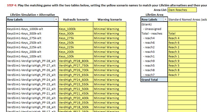
Figure 5-1. Scenario Mapping in the MMC LifeSim 2.0 Toolbox

After mapping the scenarios, consequence tables are created for each reach in the Damage Curves tab of the toolbox using the scenario and reach selections. If steady modeling is used, it may be that each reach has the same flow as the base model plan flow. However, in unsteady models the flow at each reach or gage will be different, in which case the flows must be obtained from the HEC-RAS modeler or from the project spreadsheet. If there are multiple RAS models used, you may have multiple sets of results in the same reach, but only one will be the actual results, as seen in the following figure.

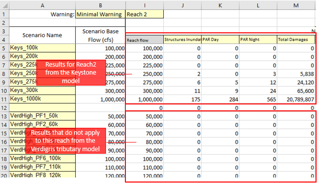
Figure 5-2. Consequences by Reach and Flow in the MMC LifeSim 2.0 Toolbox

Once the damages tab is complete, the consequences by flow tables for each reach are entered into the Damage Curves tab of the project spreadsheet located in the _Project_Speadsheet folder under the appropriate project on RMCStorage5.

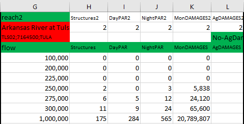
Figure 5-3. Consequences by Reach and Flow in the Project Spreadsheet

Section 5.1.5 - Review Procedures

The model is reviewed internally before consequences are considered complete. Reviews are coordinated by the MMC Production Center Consequences Branch Chief and are typically accomplished via webinar or model download.

After the products are approved by the branch chief, the economist addresses any comments. At this time, the economist uploads the finalized consequences model to the appropriate consequences folder on the MMC file share. The modeler, consequences branch chief, and team leads are informed via email of the upload and location.

Section 5.1.6 - Data Storage and Transfer

The LifeSim base and production model(s), the GIS files (structure inventory, reach polygons, etc.), and the excel files will all be uploaded to the RMCStorage5\Production\RIM\Models location in the Consequences folder under the appropriate project.

Section 6 - Web Interface Review

Section 6.1 - Web Interface Review

The purpose of the web interface review is to familiarize the district POC (the reviewer) with the RIM tool and obtain feedback regarding the data displayed in the web viewer. The GIS team member schedules and leads the webinar. The H&H modeler, H&H reviewer, H&H team lead, consequences team member, and district POC should all be in attendance.

Section 6.2 - Webinar Demonstration

The GIS team member schedules a webinar with the district POC in order to showcase the project and provide an understanding of how the RIM tool works for the district’s watershed. The GIS team member explains all of the shortcuts available that are not easily recognizable to someone who has never used the RIM tool.

Section 6.3 - Review

The reviewer ensures the data from the HEC-RAS model is displayed properly in the RIM tool by using the sliders on each reach and setting them to the various stage/flow scenarios that were modeled. The reviewer checks to ensure the inundation plotted makes sense and that, as the stages increase, the inundation also increases. The reviewer also looks at the location where two separate reaches meet to ensure the same flow is not resulting in a dramatic difference in inundation. The reviewer fills out the review checklist tab labeled “review” and ensures all of the questions are answered for the Web Interface Review section of that tab.

Section 6.4 - Address Comments

Once the review is complete, the GIS and modeling technical and team leads decide if additional items must be addressed. If comments from the review significantly change modeling or GIS data processing, the modeler or GIS team member is immediately notified to incorporate corrections. Once addressed, changes are uploaded to the RMCStorage5 drive location for the project data are uploaded to the RIM tool and submitted to the reviewer for backcheck. If no additional review is needed, the model is declared final by modeling technical lead and the following steps are taken:

• The documentation report is updated to be consistent with the model data.
• The documentation report undergoes a technical edit by the documentation team before being finalized. The modeling production process is not complete until the documentation is fully reviewed and submitted to the documentation team.
• The H&H team lead confirms the final model data was loaded into the RMCStorage5 project folder.

Section 7 - Test and Enterprise Data Loading

After the data is loaded into the local file geodatabase, the final file geodatabase is reviewed through the test website. This is done through the ArcGIS Portal and\or ArcGIS Server. This allows the contents of the database to be displayed in the test viewer and any database changes to be made prior to data loading into the enterprise database. After all comments and changes are implemented, the data is loaded into the enterprise Flood Inundation Mapping (FIM) database.

Section 7.1 - Load Testing Data into the ARCGIS Portal

The GIS team member places a copy of the fgdb data on a server accessible as a Representational State Transfer (REST) service to the RIM website via ArcGIS portal for testing. This allows the data to be immediately ready for testing. The assigned H&H lead modeler performing the QC is given a link by the GIS member who loaded the data, fills out the checklist, and returns comments to the GIS member and the database/web administrator.

Any changes to database are reloaded to the test ArcGIS portal by the GIS member and re-reviewed by the H&H lead modeler. After all issues are corrected or addressed, the data is ready for enterprise loading.

Section 7.2 - Copy Data for Enterprise Loading

The fgdb is transferred to the POC for the USACE FIM database which is a cloud-based Enterprise Oracle Spatial database. The GIS POC imports the data into a test database and, if successful, provides the file geodatabase to the MMC FIM database administrator.

Section 7.3 - Data Archive

Upon loading, all original depth grids are archived to ProjectWise (PW). Contact the GIS technical lead for location and uploading instructions.

Section 8 - Documentation and Reports

Section 8.1 - Rapid Inundation Mapping Report Workflow

The MMC documentation team places a project-specific Static Layers Development report template in the project folder on the RMCStorage5 (Production/RIM/Projects/(Basin Name)_Report). To maintain version control of the project documents, multiple copies of this report should not be created.

Section 8.2 - Modeling Team Responsibilities

The assigned modeler completes the following sections of the project-specific report:

• Executive Summary
• Hydrologic Engineering Center-River Analysis System Static Inundation Layer Development
• Reach Polygons
• Flow Increments

Additionally, the modeler fills in the engineer contact information and updates the references section with the HEC-RAS version used and any references used in the production of the report.

The modeling team lead performs a QC review of the modeling sections.

Section 8.3 - Geographic Information System Team Responsibilities

The assigned GIS specialist completes the Geographic Information System Data section of the project-specific report, fills in the GIS team member contact information, and updates the references section with the ArcGIS version used and any references used in the production of the report.

The GIS team lead performs a QC of the GIS section.

Section 8.4 - Consequences Team Responsibilities

The assigned economist completes the Consequence Data section of the project-specific report, fills in the economist contact information, and updates the references section with the LifeSim version used and any references used in the production of the report.

The consequences team lead performs a QC of the consequences section.

Section 8.5 - Document Review

The H&H team lead performs a quality assurance (QA) review of the project-specific report before notifying the documentation production lead that the report is ready for technical edit.

Section 8.6 - Documentation Team Responsibilities

Section 8.6.1 - Pre-project Setup

The MMC documentation team places a project-specific Static Layers Development report template in the project folder on the RMCStorage5 (Production/RIM/Projects/(Basin Name)_Report).

A documentation team member will fill in the cover page of the report.

Section 8.6.2 - Technical Edit and Review

After the QA, the MMC documentation team technical editor edits the document for spelling, punctuation, grammar, and content. Any issues found regarding content are directed to the assigned subject matter expert for the section.

Additionally, the technical editor corrects formatting as needed and finalizes the report.

Section 8.7 - Final Data Storage

Upon project completion, the GIS team member transfers all working files from RMCStorage5 to the final data storage located on ProjectWise.

List of Acronyms and Abbreviations

1D	one-dimensional
2D	two-dimensional
AHPS	Advanced Hydrologic Prediction Service
ArcGIS	Aeronautical Reconnaissance Coverage geographic information system
ArcMap	Aeronautical Reconnaissance Coverage map
CCP	common computation points
cfs	cubic feet per second
CWMS	Corps Water Management System
DCP	Drought Contingency Plan
DEM	digital elevation model
EPZ	emergency planning zone
ESRI	Environmental Systems Research Institute, Inc.
FEMA	Federal Emergency Management Agency
fgdb	file geodatabase
FIM	flood inundation mapping
FIS	flood insurance studies
GIS	geographic information system
H&H	Hydraulics and Hydrology
HEC	Hydrologic Engineering Center
HEC-HMS	Hydrologic Modeling System
HEC-RAS	River Analysis System
HEC-ResSim	Reservoir System Simulation
HUC	hydrologic unit code
ID	identifier
LifeSim	Life Loss Analysis
MH	maximum high
MMC	Modeling, Mapping, and Consequences
NAVD 88	North American Vertical Datum of 1988
NGS	National Geodetic Survey
NGVD 29	National Geodetic Vertical Datum of 1929
NID	National Inventory of Dams
NLD	National Levee Database
NOAA	National Oceanic and Atmospheric Administration
NSI	National Structure Inventory
NWS	National Weather Service
PAR	population at risk
PF	profile
PM	project manager
PMF	probable maximum flood
POC	point of contact
PW	ProjectWise
PWP	project work plan
QA	quality assurance
QC	quality control
REST	Representational State Transfer
RFRT	Rapid Flood Response Toolbox
RIM	rapid inundation mapping
RMC	Risk Management Center
SOP	standard operating procedures
TM	technical manual
URL	uniform resource locator
U.S.	United States
USACE	United States Army Corps of Engineers
USGS	United States Geological Survey
WSE	water surface elevation

Appendix A - Project Spreadsheet GIS Settings

The majority of the spreadsheet will be edited by the assigned H&H modeler. The following settings will be populated or verified by the GIS team member. Automated verification tools are discussed in detail in the GIS guidance document that provide quality control and data loading.

A.1 - Script Library Tab

The tab “Script LIBRARY” should be populated with the Library ID. Click on the “LIBRARY_pkid” keyword and a link will open the Basin_IDs excel spreadsheet. Once open, search for the basin name and copy the ID value to the tab’s LIBRARY_pkid “Value” cell. Lastly, the LIBRARY_date_created and Library_date_revised can be populated with first day of the month, current month, and current year when the RIM production began. If the library exists and is being revised, change the LIBRARY_revised_date accordingly.

Figure A-1. “Script LIBRARY” Tab Example Settings

A.2 - Script Settings Tab

The tab “Script SETTINGS” contains several settings unique to the user’s processing environment based on where the RIM folder storage was downloaded to for temporary processing. The root folder is the location downloaded locally from the RMC5 storage location. This folder path should contain the folder structure shown in Figure A-2.

NOTE

The “Projects” folder should be created manually and not downloaded because it contains all projects. User’s should create this folder on a local root and copy down the specific project(s) required.

Figure A-2. Downloaded System Folders for GIS Processing

The remaining values should auto-populate or remain as shown in Figure A-3.

Figure A-3. “Script SETTINGS” Tab Example Settings

Appendix B - Project Spreadsheet H&H Settings

B.1 - COE Model Info Tab

The “COE Model Info” tab is for storing the primary model information and consists of three sections: General, Steady Model Info, and Unsteady Model Info. The keywords values should be populated according to the specific project using the “Example or valid values” column as a reference. The “district_basin_field_value” will be populated from the Basin_IDs spreadsheet located in the “_software\basin_IDs” folder.

Figure B-1. “COE Model Info” Tab Example Settings

B.2 - Gage Metadata Tab

The “Gage Metadata” tab is for storing the gage identifiers associated for the entire model reach polygons and data about each gage. The gage data includes the NWS, USGS, and USACE identifiers. It also includes the “gage0”, “gage datum”, conversion values from NGVD 29 to NAVD 88, forecast information, display information, and the associated HEC-RAS river and reaches. Fill out the spreadsheet per the guidance in the readme tab and in the cell notes on each tab. One item of importance to note is how to handle ungaged and/or multi-gaged reaches.

• If more than one gage within two reaches have identical extents, but each control for a separate inflow (such as a tributary or a main stem), separate by a vertical bar (e.g., “POPW2|CRSW2”) with order downstream to upstream.
• If an ungaged reach, put controlling gages separated by an ampersand (e.g., “POPW2&CRSW2”) in order from downstream to upstream. Additional guidance is included in Sections B.2.1–B.2.3.

B.2.1 - National Weather Service Action Stage and Coordinating Flow

If available, this data can be found at https://water.weather.gov. On this site, the modeler needs to find the gage on the map. If the data is available, it should be below the graph where it will have the gage’s action stage, action flood stage, moderate flood stage, and major flood stage. If this is not available, the modeler needs to figure out the approximate stage that would be considered bank full conditions or a stage where damages would begin to occur.

B.2.2 - Gage Zero in North American Vertical Datum of 1988

This data can sometimes be found on the same webpage as the NWS action stages. If the data is not available on this page, the modeler should also try looking up the gage on the USGS webpage at the following link (user will need to include the eight digit USGS ID in place of the Xs). https://waterdata.usgs.gov/nwis/inventory/?site_no=XXXXXXXX&agency_cd=USGS.

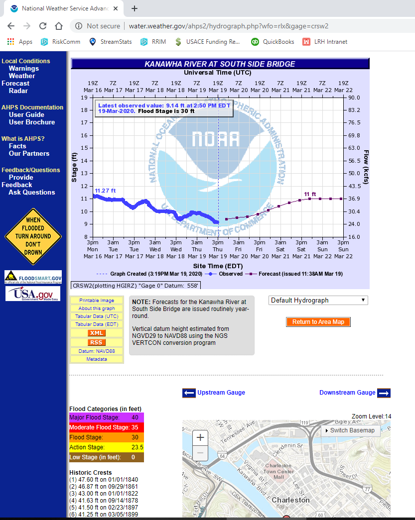
Figure B-2. Gage 0 Location from the National Weather Service Website

B.2.3 - National Geodetic Vertical Datum of 1929 to North American Vertical Datum if 1988 Datum Conversion

If the gage is in NGVD 29 or any other datum instead of NAVD 88, the modeler will need to find the conversion factor to the NAVD 88 datum. This can be found using Corpscon or other methods including survey data if available. This factor will need to be included in the project spreadsheet since the modeler will be plotting water surface elevations and all elevations will need to be in NAVD 88 datum. In order to be consistent with current standards, the gage data must be converted to the NAVD 88 datum. NOAA supports datum conversions through the work of the National Geodetic Survey (NGS). The NGS website (https://www.ngs.noaa.gov/) provides a resource for benchmarks with horizontal and vertical control nationwide and includes conversions from the current datum to NAVD 88. The NGS survey interactive map provides a means to search for current survey marks and to review survey datasheets to obtain the most up-to-date survey information. These are common references used for USGS gage locations and are appropriate for converting to NAVD 88 for use in the RIM.

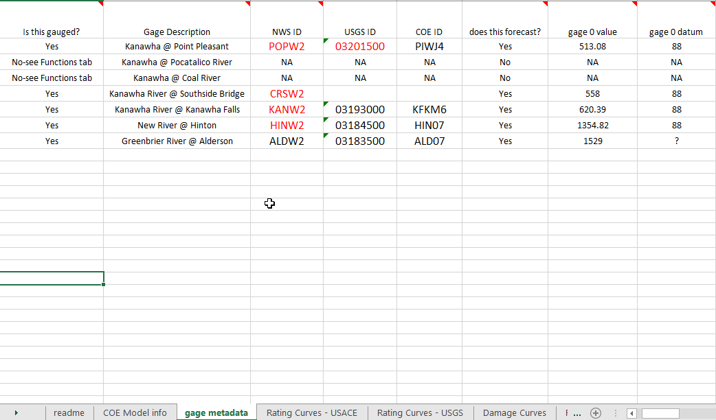
Figure B-3. “Gage metadata” Tab Example Settings

B.3 - Rating Curves-USACE Tab

The “Rating Curves–USACE” tab is for storing the USACE rating curves from the HEC-RAS model. The rating curves should only contain a one-for-one entry for each profile produced. Ensure the USACE rating curves contain only the flows produced. If the rating curve is coming from an unsteady model, it will require use of the interpolation spreadsheet to produce the rating curves that match the output profiles. Reference the instruction tab of the interpolation spreadsheet for further guidance. The interpolation spreadsheet is located at: \\wpc-netapp3.eis.ds.usace.army.mil\RMCSTORAGE5\Production\RIM\_software\interpolation_spreadsheet.

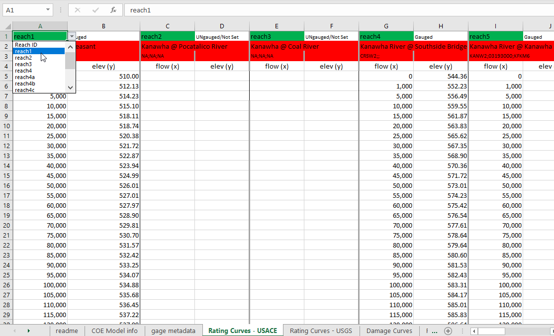
Figure B-4. “Rating Curves–USACE” Tab Example Settings

B.4 - Rating Curves-USGS Tab

The “Rating Curves–USGS” tab is for storing the USGS rating curves from the HEC-RAS model. The rating curves should only contain a one-for-one entry for each USACE WSE produced but the USGS flows do not have to match the flows from the USACE curve. If using unsteady and 2D modeling, the rating curves produced via a cross-section closest to the gage may not have a flow that matches exactly to what was produced for the output depth grids. To remedy this situation, refer to the “Interpolation” spreadsheet located in the \\wpc-netapp3.eis.ds.usace.army.mil\RMCSTORAGE5\Production\RIM\_misc folder. This tab can contain values from USACE curve combined with USGS to create a complete rating curve. A transition must exist to ensure seamless and sequentially increasing flows. The project spreadsheet ‘readme’ tab contains information on how to determine these transitions and color code them in the spreadsheet.

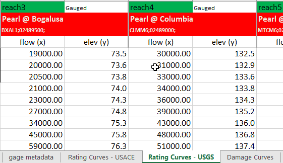
Figure B-5. “Rating Curves–USGS” Tab Example Settings

Appendix C - Reach Polygons Guidance

C.1 - Reach Polygons Template

The reach polygon template is located in the RIM\Projects\[your basin]\shp_reach_polygon\ folder.

C.2 - Delineating Inundation and Reach Polygons

The HEC-RAS modeler is responsible for creating a draft set of inundation and damage reach polygons prior to the kickoff meeting. This can be done by creating a polygon which encompasses the entirety of the HEC-RAS model geometry, then splitting the polygon at selected points. It is useful to have the following data available in GIS to facilitate the delineation of the reach polygons both prior to and during the kickoff meeting:

• Terrain (digital elevation model [DEM] or topographic lines)
• HEC-RAS model geometry (cross-sections, stream centerlines, storage areas)
• Watershed boundaries (HUC8, HUC10, and HUC12)
• River gage locations (NWS/USGS/USACE)
• HEC-ResSim Junction Points (common computation points)
• NLD and NID datasets (levee alignments and dam locations)
• Streaming maps for imagery, roads, topography, and city/town locations.

Things to consider when delineating reach polygons include:

• Watershed delineations
• Terrain changes and river slope
• Tributaries and confluences
• Known or estimated flow locations (gage points and ResSim junctions)
• Significant consequence centers
• Levees and reservoirs
• Likely extent of backwater effects up tributaries
• Storm surge influences near the coast. Each watershed is unique, and delineation of the reaches must account for a multitude of these factors. Two primary questions that should be continually evaluated during this process include:
• Will flows within this reach be relatively uniform across a large range of scenarios?
• Will data be available to estimate different flows in this reach as opposed to the adjacent reaches? During the kickoff meeting, the entire team evaluates the draft reaches polygon shapefile and edits as necessary, briefly documenting each change and the reasons for the changes in the kickoff meeting notes. If edits are made after the kickoff meeting, those changes and an updated shapefile will be provided to the entire team.

C.2.1 - Generate Polygon Extents

Reach polygons shall be created using the template files provided. These polygons represent the extents of the clipping of each flow. Each record shall contain only one polygon. The record for each shall contain:

• A field called ‘Name’ with a reach number assigned (e.g., “reach1”).
• Reaches should not have a letter—order them numerically downstream to upstream. This allows sorting in the viewer. Examples include:
• Main stem: reach1… reach 6
• Trib1 reach7…reach9
• Trib2 reach10…reach11
• All remaining fields will be filled out by GIS personnel from the Project Spreadsheet including Fields called “NWS_ID” and “USGS_ID” and “COE_ID” but the spreadsheet should be formatted in to the following specifications to ensure the reach polygon attributes are correct.
• This must be an ID that is linked to an NWS, USGS, or COE site.
• If more than one gage within two reaches have identical extents, but each control for a separate inflow (such as a tributary or a main stem), separate by a vertical bar (e.g., “POPW2|CRSW2”) with order downstream to upstream.
• If an ungaged reach, put controlling gages separated by an ampersand (e.g., “POPW2&CRSW2”) in order from downstream to upstream. The project spreadsheet is filled out with the gage IDs from other agencies. For example: a gage ID from NWS may utilize a USGS gage and should be noted. See Appendix B for guidance on populating this spreadsheet.

C.2.2 - Reach Polygon Adjustments

Figures C-1 and C-2 are examples of editing reach polygons to cut depths around inundation tributaries using the largest inundation extent (largest flow) provided.

• Ensure the polygons split in unpopulated locations unless this affects accuracy of inundation and bring in the highest flow to ensure polygons encompass the entire inundated area.
• Ensure polygons split around the inundation.

Figure C-1. Small Scale Example of Polygon Fitting around Highest Inundation

Figure C-2. Large-scale Example of Polygon Fitting around Highest Inundation